Site Report - Valley of Oaxaca

For my final project, I chose to revisit the Valley of Oaxaca dataset from a previous module assignment. I used the soil and site data from the grids N6E4, N6E5, and N6E6 to test a hypothesis concerning the rise of the Zapotec state. If population pressure was exceeding the regional carrying capacity, we would expect to see phases where the population is much greater than could be supported by agricultural yield estimates in their catchment circles. I completed this analysis with the help of ArcGIS products. Here is a basic outline of steps I created for myself to help with the         analysis process.

Methods:

1) Determine time periods to use and make into separate layers.

     - 4 time periods total

2) Buffer the sites with a 2 kilometer radius with the Buffer tool.

     - Make sure buffers are set to dissolve all.

     - 4 buffer outputs total

3) Convert the site polygons into point features using the Feature to Point tool.

     - 4 site point feature outputs total

4) Use the site points to create Thiessan Polygons for each time period.

     - 3 Thiessan Polygons total

5) Combine the site buffers with the Thiessan Polygon outputs using the Intersect tool.

     - 3 intersects total

6) Edit the intersect outputs, snapping the edges of the Thiessan polygon to the buffer and grid boundaries.

     - 3 edits total

7) Clip the soil type to the newly edited intersect outputs with the Clip tool.

     - 9 clips total

8) Calculate area in hectares of soil clips using the Calculate Geometries function.

9) Perform a spatial join between the clip layers and point file data.

     - This combines the population data with the land area data.

Based on these results, I was able to determine if the population of each site could subsist on the amount of hectares available within their 2 km catchment radius. One adult human can subsist on a minimum of .5 ha of arable land. For ease of results, 1 ha will equate to feeding 1 human

The Rosario phase settlement had an estimated population of 10, and had 192 ha of Type I land and 451 ha of Type III all arable land. With only 10-20 hectares of land required for subsistence, the Rosario phase settlement would be able to support their population on Type I land and Type III land.

The Early I phase settlement had an estimated population of 185, with 220 ha of Type I land and 1507 ha of Type III all arable land at their disposal. They would require 185 to 370 ha at most in order to sustain their population. Based on the amount of each land type available to them, they should have been able to support their population on Type I and Type III all arable land.

The Late I phase has an estimated population of 941, with only 220 ha of Type I land available, 415 ha of Type III 10% arable, and 1834 ha of Type III all arable land. They would require 941 to 1882 hectares of land at most in order to sustain their population. In terms of yield productivity, they would not have enough Type I or Type III 10% arable land to sustain their population. There would be enough Type III all arable land, but productivity and yields would not be as reliable as Type I land. 

The Monte Alban II phase had an estimated population of 774, with only 220 ha of Type I land and 1579 ha of Type III all arable land available to them. They would require 774 to 1548 hectares at most in order to sustain their population. They would not have been able to produce enough yields with Type I land. They barely meet the requirements for subsistence on Type III all arable land, which was established as not having reliable yields.

Module 11, Sharing Tools

In this lab, we corrected a few minor parameter errors in a script before successfully embedding the script into the tool for sharing. Below is a screenshot of what the tool's dialog box looks like as well as the outputs of the tool.

   

Ending notes for the semester:

Out of this whole semester,  I couldn’t pinpoint one single thing as the most interesting, as it was all (very) new and interesting to me and definitely memorable along the way (as in major stress, memorable). However, I eventually (and admittedly) enjoyed leaving my comfort zone with each successful code compilation. That being said, I expect I will use coding (of my own will) in the future.

Creating Custom Tools

This week, we created a custom toolbox and modified a script tool to go with it.

Here is what the script tool dialog box looks like.

Here is what the tool dialog window looks like after using .AddMessages() in the script.

Here is a list of the basic steps required to make a custom toolbox and script tool.

1.       Create/modify a python script.

2.       Create a custom toolbox.

3.       Add your script tool to the custom toolbox using Add>Script after right-clicking toolbox.

4.       Set the parameters of the tool in the properties to match your script.

5.       Edit your script if necessary by setting the parameters of the script using arcpy.GetParameter()

6.       Modify print statements to arcpy.AddMessage() statements to ensure messages appear in the geoprocessing environment tool dialog box.

7.       Share your toolbox, tool, and script by compressing your script and parent toolbox into a compressed (zip) folder.

Working with Rasters

In this week's lab, we worked with rasters and the arcpy.sa module. We were asked to write a code that would reassign values to an assigned raster, as well as reclassify those values to the raster. We created temporary rasters for Slope and Aspect, performed calculation statements from them, and combined the results of those calculations with the reclassified raster to create the raster output below. We created this code all within an if/else statement for checking the Spatial Analyst Extension, as these wont compile unless you have a license for it.

Here is a screenshot of my output raster below:

Here is a flowchart for my script below:

This is the step I had the most difficulty with:

1.       I had the most difficulty with the Slope and Aspects statements in part f of step 3.

2.       I kept getting only 0 (in other words, one solid color on my raster) as a result in my output raster, as it would only recognize the landcover raster.

3.       I realized I was missing my Aspect variable before the four temporary statements (I had the Slope variable already made, I guess I overlooked Aspect somehow), also I had to capitalize Slope and Aspect in the variable assignment and the four statements.

Remote Sensing

For this assignment, we classified the site Monk's Mound, located in Cahokia, Illinois. Cahokia Mounds is the largest prehistoric earthworks north of Mexico and was inhabited from ca. 600-1400 AD. It originally consisted of 120 earthworks, but today is reduced to 80. It is estimated that around 40,000 people may have lived in Cahokia at its peak, yet the reason for it's decline is still unknown. Although there is little known about Cahokia, it is still an important national landmark.

Supervised classification allows you to choose how many classes you use and their general location. I made six classes based off of what I predominantly saw in the Cahokia TIFF image. There is still some slight error in the classification, but I had more control over classification than with unsupervised.

 Unsupervised classification automatically classifies areas for you based on the number of classes you desire. This one has eight classes, with almost every single one merging into the class of another (based off toggling back and forth between images). Unsupervised is prone to more error with a fewer number of classes specified.

Writing Geometries

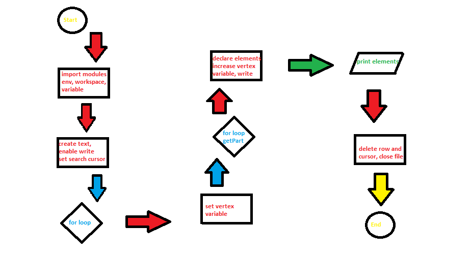
   In this lab we worked with a river shapefile, set up a search cursor with nested for loops in order to declare some of its geometries, and wrote those geometries to the text using the .write method. Below is a snip of what a portion of the text file result looks like.

Here is the flowchart of the code, with pseudocode below.

Pseudocode:

Start
Import modules
Import env
Set workspace
Set variable

Create text, enable writing
Set SearchCursor array 
For loop
Set vertex ID variable to 0
For loop/get.Part method
Element 0 of cursor array declared (feature #)
##Vertex ID printed
Element 1 of cursor array declared (x, y coords)
Element 2 of cursor array declared (name)
Vertex ID variable increased by 1
Write argument declared 
Print statement showing all five elements in single line format
Delete row and cursor
Close file

Peer Review #2

Geoprocessing tool to model beach erosion due to storms: application to Faro beach (Portugal)

 

By: Almeida, et. al

 

   This article introduces a geoprocessing tool, called GEOSTORM, which was created with the purpose of allowing users to run Kriebel and Dean’s storm erosion convolution model in ArcMap. This GIS application supports the preparation and conversion of the data produced by the model into a format usable in a GIS environment (i.e. shapefiles, etc). The application consists of two parts: Module 1, which is where the user inputs data related to their study area, and Module 2, the actual storm erosion model.

   The authors state that each module was designed with different programming languages (Python and Matlab), but do not explain the reasoning behind this. They do communicate through ArcObjects using VBA. I would like to have known if this is more or less efficient, or if it was the only way to get Kriebel and Dean’s model to run in ArcMap efficiently.

   Module 1 and 2 setup and directions are in need of more explanation. While their explanation is ok, it would not hurt to be more specific and detailed for each step the user needs to take to set up and go through the modules. The study scenario was a little unclear in some areas, and I felt like some aspects of the study could have been explained better for those outside of the discipline. Figure six is a good example and helped me better understand the results of the study.

   Overall, this application/tool sounds like it is useful and could help out coastal decision-makers prepare for incoming storms. However, the information concerning it is lacking and seems rushed out. I would like to have had more background information about the processes of each module, considering potential users would be most interested in how it works.

http://search.proquest.com.ezproxy.lib.uwf.edu/environmentalscience/docview/1675866765/abstract/9065FD92DC0B493DPQ/40?accountid=14787