Supervised Classification

In this lab, a supervised classification of current land use in Germantown, Maryland was conducted using ERDAS Imagine. AOI signatures were selected by hand using the polygon tool and recorded in the Signature Editor dialog box. All signatures were analyzed through the Mean Plot tool to determine which bands provided the greatest difference between signatures. The bands 3, 4, and 5 provided the greatest difference in signatures and was set as the band combination to reflect the data best. The signatures were then run through the Supervised Classification tool, with an additional Distance File output to show if any signature features are likely to have the wrong classification (symbolized as bright spots). The Distance File is used as a reference for correcting any wrongly classified signatures. Lastly, the supervised image is recoded by consolidating the signatures to eight classes. Those classes are agriculture, deciduous forest, fallow field, grasses, mixed forest, roads, urban/residential, and water. The final output map was created through ArcMap.

Unsupervised Classification

   In this lab, an unsupervised classification was performed on an aerial image of the UWF campus, in ERDAS Imagine, using the Unsupervised Classification tool in the Raster tab. Afterward, the results of the unsupervised classification was further reclassified by condensing the original output of fifty color categories into just five color categories. These five categories are grass, trees, shadows, roads/buildings, and mixed surfaces. Mixed surfaces is classified as pixels that can be found across multiple surface types and can not be pinpointed to just one category.

   The total area of the campus is 232.26 hectares. Of that total, 142.735 ha (61%) was classified as permeable while 89.5237 ha (39%) was classified as impermeable. Permeable surfaces consisted of the categories grass, trees, and shadows. While some shadows covered impermeable surfaces, the majority covered permeable surfaces. Impermeable surfaces consisted of roads/buildings and mixed. While some mixed surfaces covered permeable areas, the majority covered impermeable surfaces.

Thermal Imagery

The feature I identified for this lab was a large tract of bare soil located at the southern tip of the city, surrounded predominantly by urban area and some vegetation directly to the south of it. I was looking over the stretched symbology (Band 6) of the image in ArcMap when I saw a bright spot in that area, surrounded by grey (urban area) and a darker spot just below it (which looks like vegetation in the natural color image). Further analysis and comparison between the two images (natural color and thermal) determined this was bare soil. I chose to use the band combination Red- 6, Green- 3, Blue- 2. This band combination is used to distinguish between different soils and soil moisture content. The 6, 3, 2 band combination made soils appear in light to dark reds, starkly contrasting it with surrounding colors.

Image Preprocessing 2: Spectral Enhancement and Band Indices

In this lab, we used ERDAS Imagine to perform various image processing tools. Tools and topics covered were the histogram, the Inquire tool, the help menu, and interpreting features digital data. The deliverable for this assignment was to locate 3 features based on pixel variations using the directions provided in the lab. The features I located are water, ice, and water body variations. Below are my map outputs.

Image Enhancement

This lab required an attempt to remove the striping effect from a Landsat 7 image with a sensor malfunction called the Scan Line Corrector failure. In the original image, black stripes mark diagonally throughout the whole image. My final image output greatly reduced the visibility of the stripes, but slightly distorted and blurred it in some areas. I used ERDAS Imagine to enhance the image, using the Convolution, Focal Analysis, and Fourier Analysis tools. The Convolution tool, using a 3x3 sharpen kernel, lightened the stripes to white. The Focal Analysis tool was ran 6 times over the image to further lighten the stripes to a light grey. The Fourier Analysis tool was the greatest benefactor in reducing the visibility of the stripes, but as mentioned it reduced the image quality slightly.

Intro to ERDAS Imagine

The basics and navigating of ERDAS Imagine were gone over, with the end result being a portion of a subset map we were analyzing exported to be used in ArcMap. We created a new area column in the attribute table for the subset image in Imagine and exported a small portion of the image (of our choosing) to be finished in ArcMap. In ArcMap, map essentials were added, as well as a more descriptive legend concerning the extra area column we created from Imagine.

Here is my final output map:

Ground Truthing

In this lab, 30 sample points were chosen at random in order to conduct a ground truthing analysis. This analysis determined how accurate I labeled features on my map. Google Maps was the source used to confirm or deny correct identification of select features in a classification area. My Overall Accuracy was 60%.

My map output below:

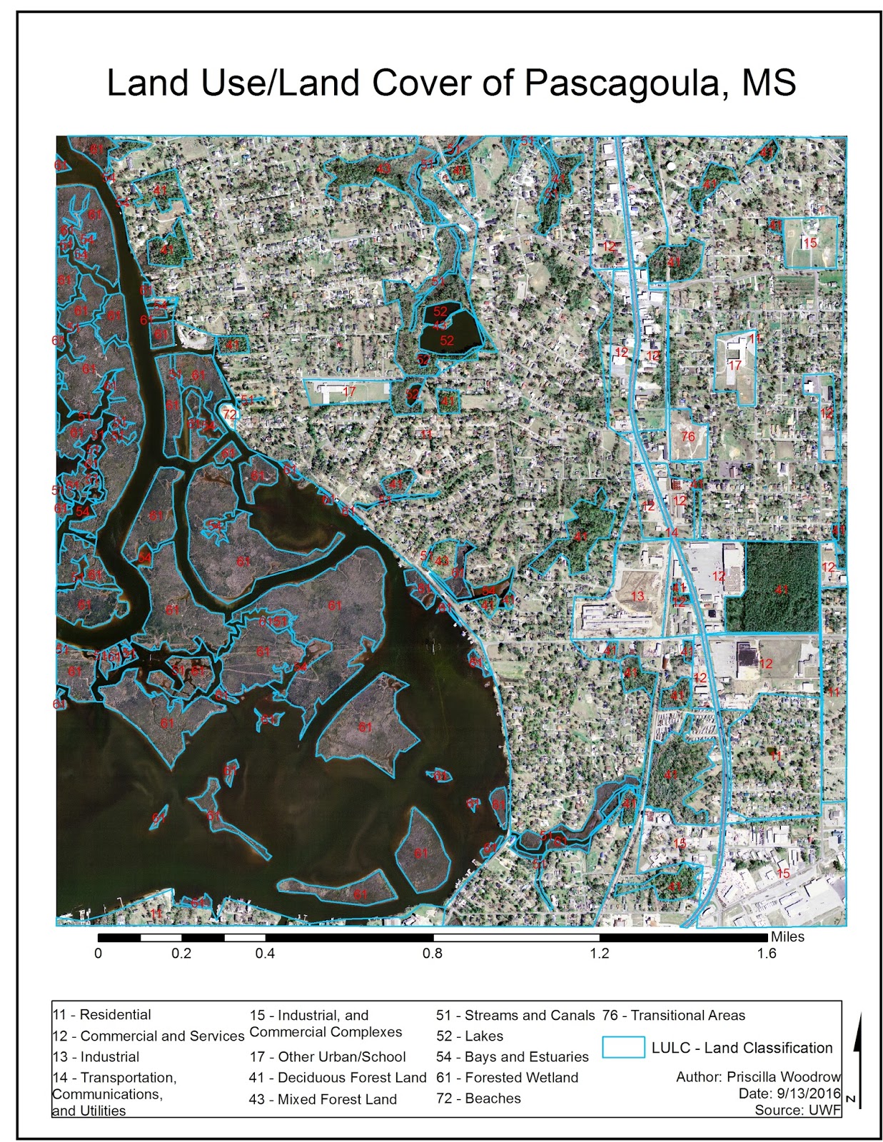
LULC Classification

This week's lab required the classification of land use and land cover of a portion of Pascagoula, MS.
The USGS Level II classification scale was used as a reference in determining how we should classify certain land types.

Here is my map outcome

Module 2 - Aerial Photography Basics & Visual Interpretation of Aerial Photography

In this lab, aerial photographs were examined and analyzed based on tones, textures, and features.

This map shows the varying tones and textures identified in the aerial photograph.

This map shows the varying patterns, shadows, shapes and sizes in the aerial photograph.