Surface Interpolation

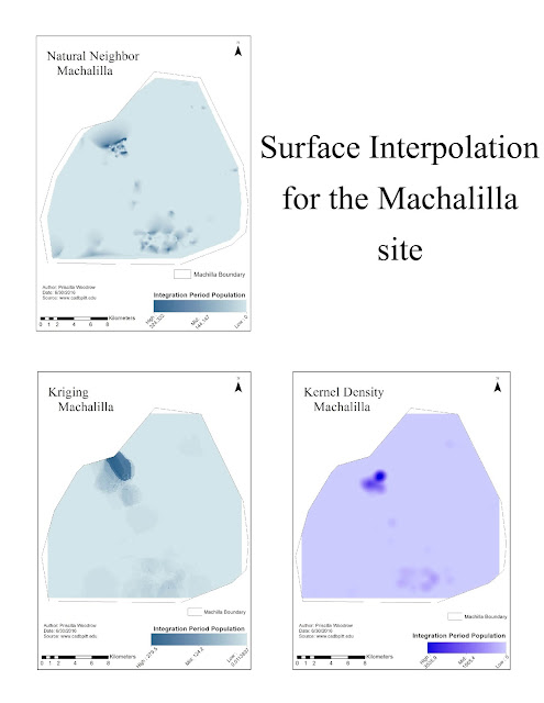
In this lab, our objective was to utilize different types of interpolation methods and to compare and contrast their uses in varying site scenarios.

This was my extra deliverable as a graduate student. This poster shows 5 different maps using varying powers of IDW interpolation. The final map on the bottom right shows the power I felt best portrayed the settlement pattern of prehispanic peoples in coastal Ecuador. This map also uses contouring to highlight the areas with a larger population.

This poster shows the varying density maps I used to portray population density at the Barriles site.

This maps shows the varying density maps I used for the Machalilla site.

Exploring and Manipulating Spatial Data

Here is the general flow of my code:

Hardest part of the assignment for me:

       I had the most difficulty with step 7 (creating a for loop to populate the dictionary). I was under the impression that a separate for loop had to be made in order to populate the dictionary. I was able to print out the cities with the population underneath them alright, but my list would not appear at the end of the results when I tried adding another for loop underneath (completely separate from) my search cursor code.

       The solution was to simply add the dict.update function in the for loop of the previous code where I conducted a search for the fields I was trying to isolate. The rows (AKA fields), not the field names, are integral in performing the update to the dictionary, I found out.

Here is the results of my script:

In this lab, we had to create a code that would make a new geodatabase in our results folder, search for certain fields in one shapefile's attribute table, and display those fields by populating an empty dictionary with the results.

The screenshot shows the shapefiles that were copied into the geodatabase and print messages stating when a certain part of the process was completed. It prints that the search for the certain attribute table fields is underway and also that it completed. Finally, it prints a message that the dictionary is being updated and completed, with results of the dictionary underneath. 

Digitizing, Module 6

   In this lab, we georeferenced old maps of archaeological sites and land cover to Oaxaca Valley, Mexico. In addition to that, we created shapefiles for and digitized the land cover and archaeological sites for each grid. Finally, we were to join tables of our digitized sites to a prepared excel file. My grids were N4E3, N4E4, and N4E5. 

This is a map of my three georeferenced grids. The most difficult part of this assignment was determining the grid locations. The historical topographical map I was georeferencing was especially blurry in the location of my grids, so you see that they do not line up perfectly.

 These next three maps show each grid and its digitized features. This part of the assignment was not difficult, but very time consuming. However, it was hard to read and determine the labels on some of the site features.

 This map shows the population estimate for a Monte Alban IIIB site in my N4E5 grid. The assignment was to find the most densely populated IIIB site cluster and symbolize it according to the low population field in the attribute table. However, I only had one IIIB site out of all my grids, with a low pop of 10. The site is located in an all arable land type, but is far from a river. I can only guess that even though it was on good land, it must have been isolated in some way from other resources.

Geoprocessing with Python

Steps I took to make my script:

1.       I imported arcpy, set the workspace environment to the module 6 data folder, and set the overwrite output environment to true.

2.       I set the hospitals shapefile as a variable (input_feature) in order to be added to the map.

3.       I made a try statement comprised of three components. The first component adds the hospitals using the AddXY management tool with the hospitals set as the variable ‘input_feature’. The second adds a buffer of 1000 meters to the hospitals and saves the output into my results folder. The third dissolves the hospitals buffer and saves the results into my results folder. All three components get a print messages statement directly after their implementation. This shows a message that the tool ran and details about its process.

4.       Last I incorporated an except statement that would print the message “An error has occurred.” if any of the above processes fail.

This shows the flow of my script.

Here, the print statements display the messages left by the tools after running.

Geoprocessing with ArcGIS

   In this weeks lab, our objective was to create a toolbox, create a model in that toolbox, and export the model into a script that is usable outside arcmap.

   This flowchart shows the process of how the model-turned -script is run.

   This is what the outcome of the model looks like. The model took two shapefiles (basin and soils), and used the Clip tool to clip the soil type to the basin. Next, the Selection tool was used to select not prime farmland out of the soil types in the basin. Finally, the Erase tool was used to erase the not prime farmland from the basin polygon.

   Here are the steps I took to create the Erase function in my model:

1.       I dragged the Erase tool into my model.

2.       I double-clicked the tool to bring up the dialog box.

3.       I set the Input Features as basin and the Erase Features as my Select_Soils selection. I named the Output Feature Soil_Erase.

4.       I right clicked the Output Feature in the model and clicked Add To Display.

5.       I ran the process. I unchecked the display of all other layers in the dataframe except the Soil_Erase to ensure that the Not Prime Farmland was indeed erased from the basin.

Peer Review Assignment 1

Development of Python-FALL3D:

a modified procedure for modelling volcanic ash dispersal in the Asia-Pacific region

By: A.N. Bear-Crozier, Nugraha Kartadinata, Anjar Heriwaseso, Ole Nielsen

http://link.springer.com/article/10.1007/s11069-012-0273-7  (abstract)

This article talks about the simplification of a volcanic ash dispersion model called FALL3D. This modelling program is already widely used by many countries, such as Italy and Iceland, who experience volcanic activity periodically. However, FALL3D requires extensive experience and background knowledge of computational modelling to run properly. Individuals with experience such as this is lacking in developing countries such as Indonesia, a major volcanic hotspot in need of a volcanic ash dispersal modelling program.

The solution presented by the authors was the development of a script written in the Python coding language that modifies the procedures that run the modelling program. This script, called Python-FALL3D, automatically streamlines the installation process and makes inputting and processing data simplified throughout the code by allowing the user to execute each process in single-steps. This allows those with little or no background in computational modelling to use this program.

The research conducted behind the benefits and limitations of this script are conclusive and honest. The developers have thoroughly tested FALL3D in other volcanic ash hazard regions with good results and are positive that its application can be put to use in the Asia-Pacific region. Contrarily, while the program itself is simplified, it is still dependent upon several other factors, such as internet connectivity, experience using the Linux operating system, and its codependency on other complex programs in order to operate correctly. As mentioned earlier, individuals with experience running programs like these are lacking in developing countries, and access to a reliable internet connection may not be possible in some regions of Asia-Pacific.

The developers do an excellent job explaining the installation process as well as methods of collecting and preparing meteorological data relevant to the region. They provide an applicable scenario displaying the computational models’ efficiency by simulating the volcanic ash hazard of the active volcano Gunung Gede, in West Java, Indonesia. The processes underlying the script along with a scenario of its theoretical application are in tangent with each other, and the charts and figures greatly enhance the understanding of the process and results.

 In theory, the application of Python-FALL3D in the Asia-Pacific region would immensely aid cities in close proximity of active volcanoes by being able to forecast volcanic ash landfall direction and speed. The fact that it is also available free and open source to download show the willingness and dedication of its creators to make the script available to those who need it. The only drawback I can see is the actual usability this program will receive in the Asia-Pacific region due to aforementioned factors.

Georeferencing, Mod 5

   In this lab, we georeferenced a historical map of Macao (present day Macau), created by explorer James Cook and published in 1785. Macau is located nearby Hong Kong, China and is a popular tourist location. The image was downloaded from the David Rumsey Historical Map Collection website. I georeferenced the historical map to a present day basemap by selecting control points on each map to connect to one another. The historical map is distorted due to 'historical' inaccuracies concerning actual island locations and present day differences. However, I based my control points off of still existing features, such as elevation points (with the help of a topography basemap), and was able to get the historical map to represent present day Macau as close as I could.

Debugging and Error Handling

   This script contained a few syntax errors that prevented it from listing the field names in the attribute table of a shapefile.

    This script contained syntax errors, incorrect pathfile locations, incorrect methods, and I had to adjust the parameters of a method. It lists the layers found in this module's map document.

    This script incorporates a try/except statement to catch an exception, instead of fixing the errors. Catching an exception bypasses the error statement when trying to run the code and instead prints out  the main issue. The second part of the script runs successfully and lists the name of the data frame, the set spatial reference of the map document, and the scale of the map document.

   This flowchart shows the process of the second script (second screenshot).

   This is how I incorporated a try/except statement into the third script:

1.      I added ‘try:’ to the top of the code, highlighted the rest and tabbed it.

2.      I added ‘except Exception as exc:         print “An error has occurred.”            Print exc          to the bottom of the code as shown in the mod 4 lecture.

3.      I only did this for Part A, as the directions for Part B said it would run successfully.

Historic, Module 4

   The purpose of this module was to acquaint us with online resources of historic information and how to locate and interpret historical records on these sites. In the lab we learned how to hyperlink the historical images seen on the map into a point shapefile of Paul Revere's house location in the city of Boston.

   This map was created for the purpose of illustrating historic Boston and the location of Paul Revere's home. Included on the map is an image of Paul Revere, a star point indicating his home location, and an image of a census count with his name listed on it. Below is a short description of who Paul Revere is and what he is known for. Also included is the URL to the Google Map location of his home in Boston.